Paper 6 A Bayesian Lasso via reversible-jump MCMC

Chen, Wang, and McKeown (2011)

6.1 先验：标题党：

• 怎么在Bayes问题中使用Lasso penalty，是如原文中所说的Laplace prior吗？如何抽？
• Reversible-Jump MCMC是什么，该去看哪篇文章
• 细节：略过，因为是signal processing的，总感觉不是统计的。。。

6.2 Abstract:

In this paper, we propose a new, fully hierarchical, Bayesian version of the Lasso model by employing flexible sparsity promoting priors, A reversible-jump MCMC algorithm is developed for joint posterior inference over both discrete and continuous parameter space.

号称比Optimization-based，Gibbs sampler-based and Binomial-Gaussian prior model，有更精确，更准确地sparsity 特征。

在diabetes数据上和fMRI数据上进行了跑分。 Extension：MCMC-based algorithm for Binomial-Gaussian estimate via simulations。

因为涉及到fMRI data感觉如果可能的话得找代码跑一遍看看

6.3 Introduction

6.3.1 Sparse linear models:

\[ \mathbf{y}=X \boldsymbol{\beta}+\mathbf{e} \] 对于fMRI data维度诅咒很常见，Multivariate autogregressive models(mAR) 是常见的对fMRI建模的方法。 但是，在fMRI data的实践中，如果使用传统的full mAR 对大脑之间的联系，当ROIs（感兴趣的区域）节点数远大于时间节点数的话，模型提取信息的能力会下降。（break down） 目前，考虑20个ROIs ，那么每当mAR模型的阶数加一，则会出现额外的400个参数需要确定。然而观测数则很少。

因为涉及fMRI所以稍微写细一点

处理cod（curse of dimensionality)的一个方法就是降维。In the example of modelling brain networks using fMRI, this variable selection procedure could significantly reduce the number of edges in the learned networks, resulting in sparse connectivity networks.

以下这段和统计好像无关，signal processing 上的。 Sparse linear approximation of a signal from a set of overcomplete dictionary is also an intensive research topic in both the signal processing and compressed sensing literature. basis pursuit.

“spike and slab” priors on the regression coefficients were proposed in (Mitchell and Beauchamp 1988)

Using the Laplace or Bernoulli–Gaussian mixture prior on the regression coefficients and introducing latent variables to identify subsets have been the popular choice.

This paper propose a fully Bayesian Lasso framework with the RJ-MCMC approach.

Variable/model selection methods, penalized regression approach, a easy to implement framework by Fan et.al. (2004).

Lasso in Bayesian, posterior mode with Laplace (double-exponential) prior. D. Hunter, R. Li (2005) proposed Minorize-Maximize algorithm, to transfer the problem of maximizing the posterior function. “the Laplace prior to sequentially maximizing its quadratic surrogate functions.”

Several Laplace-like priorhas veen recently proposed.[37] Mixture of delta-mass, Jeffrey’s non-informative mixing distribution.[10] This paper employ a Laplace prior for regression coefficients and implement it as RJ-MCMC-based approach. [27]“The Bayesian lasso”.

6.3.2 Related work and our contribution

Tuning parameter, usually selected by minimize the generalized CV erros. As a full Bayesian approach with Laplace prior on \(\beta\), giving the shrinkage tuning parameter a prior and the posterior of the model can be derived by integrating parameters via its posterior distribution. In this occasion, the proposed Bayesian Lasso estimator has a different posterior distribution from the ordinary Lasso with Laplace prior.

Motivated by [24,37], two extra parameters in the proposed Bayesian lasso model to separately control the model selection and estimation shrinkage issues. Poisson prior on the model size together with Laplace prior on \(\beta\). Joint posterior distribution is highly non-standard and a standard MCMC is not applicable, employ RJ-MCMC than.

6.3.3 Notations

\(\gamma\), p-length binary vector denote the zero or nonzero coefficients.

6.4 A fully Bayesian Lasso model

6.4.1 2.1. Prior specification

Independent Laplace prior are assumed for \(\beta\), with correspond active set \(\boldsymbol \gamma\) with \(|\boldsymbol\gamma|=k\) with follows the distribution \[ \pi\left(\beta_{j} | \tau, \gamma\right)=\frac{1}{2 \tau} \exp \left(-\frac{\left|\beta_{j}\right|}{\tau}\right) \] Since how much should be shrinkage is unkown, a non-informative prior is given to hyper-parameter \(\tau\). By same reason,also give a non-informative prior to variance of noise \(\sigma^2\)

Due to the Lindley’s paradox, one needs to be very careful to assign improper priors for \(\tau\) or \(\sigma^2\)

Furthermore, prior probabilities are also assigned to eachpossible sub-model, that is, a sub-model containing k predictors follows a right-truncated Poisson distribution at p.

\[ p(k | \lambda)=\frac{e^{-\lambda} \lambda^{k}}{C k !} \]

Therefore, the posterior distribution of the parameter vector

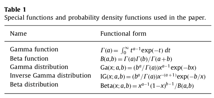
\[ \begin{array}{l}{p\left(\boldsymbol{\beta}, \tau, \sigma^{2}, \gamma, \lambda | \mathbf{y}, X\right) \propto \frac{e^{-\lambda} \lambda^{k-1}}{\left( \begin{array}{c}{p} \\ {k}\end{array}\right) k !} \tau^{-(k+1)} \sigma^{-(n+1)}} \\ {\exp \left(-\frac{\|\boldsymbol{\beta}\|_{1}}{\tau}-\frac{\|\mathbf{y}-X \boldsymbol{\beta}\|_{2}^{2}}{2 \sigma^{2}}\right)}\end{array} \] Derive detail can be found in Appendix. To reduce the computational cost, the parameters \(\tau,\sigma^2\) and \(\lambda\) can be analytically integrated out. Normalization constants of the respective Gamma and inverse Gamma p.d.f’s, we can show that

\[ \pi(\boldsymbol{\beta}, \gamma | \mathbf{y}, X) \propto \Gamma(k) B(k, p-k+1)\|\boldsymbol{\beta}\|_{1}^{-k}\|\mathbf{y}-X \boldsymbol{\beta}\|_{2}^{-(n-1)} \] This equation has two parts, \(||\boldsymbol\beta||_1^{-k}\) is the prior information and \(\|\mathbf{y}-X \boldsymbol{\beta}\|_{2}^{-(n-1)}\) is the likelihood. By integrating out the nuisance parameters analytically, a more stable estimator is possible, in addition to the advantage of requiring fewer computations.

6.5 Bayesian computation

Algorithm

The proposed RJ-MCMC based Bayesian Lasso

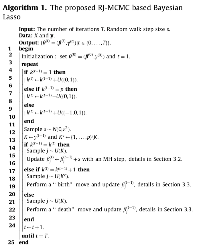
没解说直接看怎么感觉有点像MH，需要一点解说

Propose a hybridized MCMC sampler to simultaneously perform model averaging and parameter estimation and falls into the RJ-MCMC umbrella.

6.5.1 Design of model transition.

Disribution of \(\beta\) depends on the model dimensionality. Here, we propose three types of model moves as following:

\[ \text { 1. } \gamma \rightarrow \gamma ; \quad \text { 2. } \gamma \rightarrow \gamma^{\prime} ; \quad 3 . \gamma^{\prime} \rightarrow \gamma \]

看不懂，得看看hybridized MCMC是啥 (Brooks, Giudici, and Roberts 2003) may be need to check about this MCMC methods.

6.5.2 A usual Metropolis-Hastings update for unchanged model dimension

Proposal used: Gaussian random walk (RW) is used, with acceptance probability with \[ \min \left\{\left(\frac{\left\|\boldsymbol{\beta}^{\prime}\right\|_{1}}{\|\boldsymbol{\beta}\|_{1}}\right)^{-k} \times\left(\frac{\left\|\mathbf{y}-X \boldsymbol{\beta}^{\prime}\right\|_{2}}{\|\mathbf{y}-X \boldsymbol{\beta}\|_{2}}\right)^{-(n-1)}, 1\right\} \]

6.5.3 A birth-and-death strategy for changed model dimension

For the model jumping moves, there are two commonly used proposals:

• birth-and-death
• split-and-merge

birth-and-death is a simple form of model transformation: in the birth step, a new predictor is added to the current model, by generating parameters of a new predictor from a prior distribution. In the death step, a predictor is removed from current model, and the reversibility constraint must be satisfied according to the detailed balance equation.

然后似乎是要满足什么条件，又看不懂了。(Green 1995) 如果有需要的话感觉得查查原文

还有一点不懂，这个birth-and-dead 过程类似于前向和后项选择过程，是怎么和Bayes lasso扯上关系的，感觉有点像LARS的solution path方法

6.6 Simulation

run for 100,000

References

Chen, Xiaohui, Z. Jane Wang, and Martin J. McKeown. 2011. “A Bayesian Lasso via reversible-jump MCMC.” Signal Processing.

Mitchell, T J, and JJ Beauchamp. 1988. “Bayesian variable selection in linear regression.” Journal of the American Statistical Association, 1023–32.

Brooks, S P, P Giudici, and G O Roberts. 2003. “Efficient construction of reversible jump Markov chain Monte Carlo proposal distributions.” Journal of the Royal Statistical Society: Series B (Statistical Methodology) 65 (1): 3–55.

Green, Peter J. 1995. “Reversible jump Markov chain Monte Carlo computation and Bayesian model determination.” Biometrika 82 (4): 711–32.